A lot of MATLAB’s conveniences over Python and vice versa stem from their design choices of what are first class citizens and what are afterthoughts.
MATLAB has its roots from scientific computing, so operations (use cases) that are natural to scientists come first. Python is a great general purpose language but ultimately the motivation came from a computer science point of view. It will eventually get clumsy when Python tries to do everything MATLAB does.
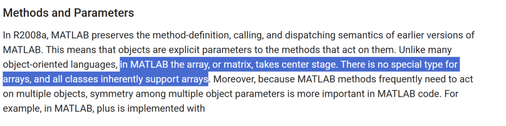
Matrix (a stronger form of array) takes the center stage in MATLAB
In MATLAB, matrix is a first-class citizen. Unlike other languages that starts with singleton and containers are built to extend it to arrays (then to matrices), nearly everything is assumed to be a matrix in MATLAB so a singleton simply seen as a 1×1 matrix.
This is a huge reason why I love MATLAB over Python based on the language design.
Lists in Pythons are cell containers in MATLAB, so a list of numbers in Python is not the same as an array of doubles in MATLAB because the contents of [1, 2, 3.14] must the same type in MATLAB.
Non-uniform arrays like cells/lists are much slower because algorithms cannot take advantage of uniform data structure packed very locally (the underlying contents right next to each other) and do not need extra logic to make sure different types are handled correctly.
np.array() is an after thought so the syntax specifying a matrix is clumsy! The syntax is built on lists of lists (composition like arr[r][c] in C/C++). There used to be a way to use MATLAB’s syntax of separating rows of a matrix with a semicolon ‘;’ with np.matrix('') through a string (which clearly is not native and code transparent).
Given that np.matrix is deprecated, this option is out of window. One might think np.array would take similar syntax, but heck no! If you typed a string of MATLAB style matrix syntax, np.array will treat it as if you entered an arbitrary (Unicode) string, which is a scalar (0 dimension).
For my own use, I extracted the routine numpy.matrix used to parse MATLAB style 2D matrix definition strings as a free function. But the effort wasted to get over these drivels are the hidden costs of using Python over MATLAB.
import ast

'''
mat2list() below is _convert_from_string() copied right off
https://github.com/numpy/numpy/blob/main/numpy/matrixlib/defmatrix.py
because Numpy decided to phase out np.matrix yet choose not to
transplant this important convenience feature to ndarray
'''

def mat2list(data):
    for char in '[]':
        data = data.replace(char, '')

    rows = data.split(';')
    newdata = []
    for count, row in enumerate(rows):
        trow = row.split(',')
        newrow = []
        for col in trow:
            temp = col.split()
            newrow.extend(map(ast.literal_eval, temp))
        if count == 0:
            Ncols = len(newrow)
        elif len(newrow) != Ncols:
            raise ValueError("Rows not the same size.")
        newdata.append(newrow)
    return newdata
Numpy array is really cornering users to keep track of the dimensions by providing at least 2 pairs of brackets for matrices! No brackets = singleton, 1 pair of brackets [...] = array (1D), 2 pairs/levels of brackets [ [row1], [row2], ... [rowN] ] = matrix (2D). Python earns an expletive from me each time when I type in a matrix!
Slices are not first class citizens in Python
Slices in Python are roughly equivalent to colon operator in MATLAB.
However, in MATLAB, the colon operator is native down to the core so you can create a row matrix of equally spaced numbers without surrounding context. end keyword, as a shortcut to get the length (which happen to be the last index due to 1-based indexing) of the dimension when indexing, obviously do not make sense (and therefore invalid) for colon in free form.
Python on the other hand, uses slice object for indexing. Slice object can be instantiated anywhere (free form) but buidling it from the colon syntax is exclusively handled inside the square brakcet [] acess operator known as the __getitem__ dunder method. Slice objects are simpler than range as it’s not iterable so it’s not useful to generate a list of numbers like colon operator in MATLAB. In other words, Python reserved the colon syntax yet does not have the convenience of generating equally spaced numbers like MATLAB does. Yuck!
Since everything is a matrix (2 dimensions or more) in MATLAB, there’s no such thing as 0 dimension (scalar) and 1 dimension (array/vector) as in Numpy/Python.
Transposes in Python makes no sense for 1D-arrays so it’s a nop. A 1D-array is promoted into a row vector when interacting with 2D arrays / matrices), while slices makes no sense with singletons.
Because of this, you don’t get to just say 3:6 in Python and get [3,4,5] (which in MATLAB it’s really {3,4,5} because lists in Python are heterogeneous containers like cells. The 3:5 in MATLAB gives out a genuine matrix like those used in numpy).
You will have to cast range(3,6), which is an iterator, into a list, aka list(range(3,6)) if the function you call with it does not recognize iterators but instead want a generated list stored in memory.
This is one of the big conveniences (compact syntax) that are lost with Python.
More Operator Overloading
Transposes in Numpy is an example where CS people don’t get exposed to scientific computing enough to know which use case is more common:
| MATLAB | Numpy | Meaning |
a.' | a.transpose() or a.T | transpose of a |
a' | a.conj().transpose() or a.conj().T | conjugate transpose (Hermitian) of a |
Complex numbers are often not CS people’s strong suit. Whenever we do a ‘transpose’ with a physical meaning or context attached to it, we almost always mean Hermitian (conjugate transpose)! Most often the matrix is real anyway so many of us got lazy and call simply call it it transpose (a special case), so it’s easy to overlook this if one design/implement do not have a lot of firsthand experience with complex matrices in your math.
MATLAB is not cheap on symbols and overloaded an operator for transposes, with the shorter version being the most frequent use case (Hermitian). In Python you are stuck with calling methods instead of typing these commonly used operators in scientific computing like they are equations.
At least Python can do better by implementing a a.hermitian() and a.H method. But judging that the foresight isn’t there, the community that developed it are likely not the kind of people sophisticated enough in complex numbers to call conjugate transposes Hermitians.
Conventions that are more natural to scientific computing than programming
Slices notation in Python put the step size as the last (3rd) parameter, which makes perfect sense from the eyes of a programmer because it’s messy to have the second parameter mean step or end point depending on whether there’s one colon or two. By placing the step parameter consistently as the 3rd argument, the optional case is easier to program.
To people who think in math, it’s more intuitive when you specify a slice/range in the order you draw the dots on a numbered line: you start with a starting point, then you’ll need the step-size to move onto the next point, then you’ll need to know when to stop. This is why it’s start:step:stop in MATLAB.
Python’s slice start:stop_exclusive:step convention reads like “let’s draw a line with a starting point and end points, then we figure out what points to put in between”. It’s usually mildly unpleasant to people who parse what they read on the fly (not buffering until the whole sentence is complete) because a 180 degree turn (meaning reversed) can appear at the end of a sentence (which happens a lot with Japanese or Reverse-Polish-Notation).
Be careful that the end points in Python’s slice and C++’s STL .end() are exclusive (open), which means the exact endpoint is not included. 0-based index systems (Python an C++) love to specify “one-past-last” instead of the included end points because it happens to align with the total count N: there are N points from [0, N-1] (note N-1 is inclusive, or a closed end) which is equivalent to [0, N), where N is an open end, for integers. This half-open (or open-end) convention avoids painfully typing -1 all over the place in most use cases in a 0-based indexing system.
0-based indexing is convenient when doing modulo (which is more common with programmers) while 1-based indexing matches our intuition of natural numbers (which starts from 1, bite me. lol) so when we count to 5, there are 5 items total. My oscilloscope don’t call the first channel Channel 0 and I work with floats more than I work with modulo, so 1-based indexing has a slight edge for my use cases.
MATLAB autoextends when assigning index out of range, not Python
This is one behavior I really hated Python for it, with passion. Enough for me to keep MATLAB in parallel with Python instead of ditching MATLAB completely.
In MATLAB, I simply assign the result x{3} = 4 even when the list x starts with an empty cell x={} and MATLAB will be smart enough to autoextend the list. Python will give you a nasty IndexError: list assignment index out of range.
I pretty much have to preallocate my list with [None] * target_list_size. MATLAB are pretty tight-assed when it comes to not allowing syntax/behaviors that allow users to hurt themselves in insidious ways, yet they figured if you expanded a matrix that you didn’t intend to, soon you’ll find out when the dimensions mismatch.
Note that numpy array has the same behavior (refuses to autoexpand array when assigned an index out of the current range).
No consistent interface for concatenation in Python
In MATLAB, if you have a cell of tables C, you can simply vertically concatenate them simply with vertcat(C{:}), because MATLAB has a consistent interface for vertical concatenation, which is what the operator [;] calls.
Note that cell unpack {:} in MATLAB translate to comma separated list, putting a square bracket over commas like as [C{:}] is horzcat(C{:}) because it’s [,].
Python doesn’t have such consistent interface. Lists are concatenated by + operator while Dataframes are concatenated by pd.concat(list_or_tuples_of_dataframes, ...), as + in Dataframes means elementwise application of + (whatever + means to the pair of elements involved).
I just had a simple use case where I have a list containing dataframes corresponding to tests on each channel (index) that I’ll run the experiments on one by one. They don’t need to be run in order nor all of the tests need to be completed before I collect (vertically stack) the dataframes into one big dataframe!
Vertically stacking such a list of Dataframes is a nightmare. Pandas haphazardly added a check that throws an error for pandas.concat() if everything in the list is None, which throws an error “ValueError: All objects passed were None“!
If I haven’t run any tests yet, attempting to collect an aggregrate table from all empty tables should return None instead of throwing a ValuerError! Checks for attempting to do a nop depending on the source data should be left for users! It’s safer to do less and let users expand on it than nannying and have users painfully undo an unwanted goodwill!
How empties are handled in each data type like cell or table() is a important part for a consistent generic interface to make sure different data type work together (cast or overload automatically) seamlessly. TMW support showed me a very detailed thought process on what to do when the row is empty (length 0) or column is empty (length 0) in our discussion getting into the implementation details or dataset/table (heterogenous data type). I just haven’t seen the thoughtfulness in Python (lists), Numpy (array) or Pandas (dataframe) yet.
Now that with the poorly thought out extra check in pd.concat(), I have to check if the list is all None. I often do not jump to listcomp or maps if there’s a more intuitive way as listcomps/maps are shorthands for writing for-loops instead a expressing specific concept, such as list.count(np.nan)==len(list) or set(list)=={'None'} for checking if all entries in the list are NaN or None. Both of them are no-go because:
- Dataframe broke
list.count()withTypeError: unhashable type: 'DataFrame'because Dataframe has no__hash__, because it’s mutable (can do in-place operation through reference).
- Then dataframe breaks
set()withValueError: The truth value of a DataFrame is ambiguous..., because the meaning of==changed from object comparsion (which returns a simple boolean) to elementwise comparsion (that returns a non-singleton structure with the same shape/frame as the Dataframe itself).
![]()