When programming C++, I have prefer to stick to free functions and refactor everything generic into libraries. However it doesn’t sound like the norm for now. I’m glad after sawing this video that that I’m not the only one who prefers free functions.

This lecture explains why prefering free functions instead of jumping to cram everything into classes aligns with OOP doctrines, but that’s not how I came up with this idea on my own.

TLDR: My whole thesis of preferring free functions is based on

1. there’s no reason to reinvent the wheel badly by not identifying generic operations and factor it out as calls to generic libraries not tied to the business logic!
2. my observation that data mambers are globalist (global variable) style of programming sugarcoated by containing the namespace pollution with class scopes!

The lecture suggested putting some part of business logic code as free functions too, right after class definitions. I didn’t really think of that because I often refactor aggressively enough that there’s not much left to pollute the class’s namespace.

If you can refactor your code very well, the top level code should be so succinct that it pretty much reads the business logic without the noise from implementation details, to the extent that non-programmers can develop a picture of what your code does without knowing the intricate mechanics of the programming language.

---

Background

Class is a mental model built on Von Neuman architecture suggesting that data (variable) and program (functions) aren’t very different after all.

Structs provides a compact way to bundle different variables into one logical unit. It’s more of an eye candy.

Given the Von Neuman’s view that program (function pointers in reality) is treated as a data (variable), a struct can bundle programs and data.

Then people naturally made up the fabric of classes, calling a bundle of actions (program) anda state (data) an object to mimic our daily observations.

Making certain variables (fields) in struct callable requires a little special treatment that could be done in the compiler. This is the very primitative form of classes.

I said state here because data members in OOP naturally encourage people to frame the program in terms of shared states instead of tightly controlled data flow by passing arguments in function calls.

Functional programming avoids states which makes it a polar opposite way of structuring your program and data structures than OOP. It’s not even passing data, but chain acting on data.

---

Direct delivery (local variables) vs Sharing access (data members)

Shared states is what globalist programmers (pun intended) are doing with non-local variables.

With local variables passed through arguments in function calls, you hand the item (say a letter) to the intended recipient (the function you call) directly. It’s point-to-point delivery: simple and predictable.

With data members or nonlocal variables, you leave your message in the dropbox (non-local scope or data member scope) and hope for the best (the right people will pick it up and nobody messed with it in between).

People say globals are evil, but they are missing the point by thinking it’s just the breadth of namespace pollution that makes it evil. It’s actually the dropbox mechanism that make your program fragile and defenseless against domestic (namescope) violence (unwanted data mucking).

Enclosing globals into data members only limits the potential public violence into potential domestic violence (pun intended).

Classes merely put a lock in the dropbox and give ALL people in the same family/Class (methods) the same key for private members. Public means unlocked.

Think of data members scope as a fridge at home. Methods are the people at home. Whoever that has the home key can put food in the fridge, mess with it, or eat it.

Within the same class/family, there are no finer controls over who (methods) can touch which food item (data member) as long as they are in the same trusted level.

So if you didn’t refactor your class composition (not hieracy, as hierachy likely exposes more data members to more methods that doesn’t need it) to only allow intended methods to access only the data members they need, you are not encapsulating tightly.

“Only allow intended methods to access only the data members they need” is hell of hard. This is the same as saying that you need to devise a complicated composition hieracy and manage the interfaces between them so every class involved is a complete bipartite graph between data members and methods!

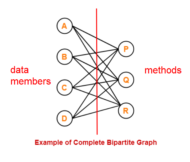
For example, if method R only needs (A,B,C), it should not have access to D, so D needs to be factored out into another class. If data member B is needed only by methods (P,Q), it should not be in the same family as R. Then you have to manage the interfaces between these classes. Yikes!

If you get this far to encapsulate properly, you might as well factor as many method as you can into directly passing variables in free functions. In reality we don’t really go this far and stop somewhere when the bipartite graph is dense enough so our mind can keep track of all possible parties (which methods are involved with what data members) within the class.

---

Compromise / Solution?

There are applications like GUI objects that it’s just a total pain in the ass to explicitly pass data through arguments over every event (callback) so state holding (data members) makes more sense. Eventually we need to leave something to data members even if we did our best to factor free functions out of the class. GUI is one of the use cases where I won’t shame myself for abusing non-local scopes.

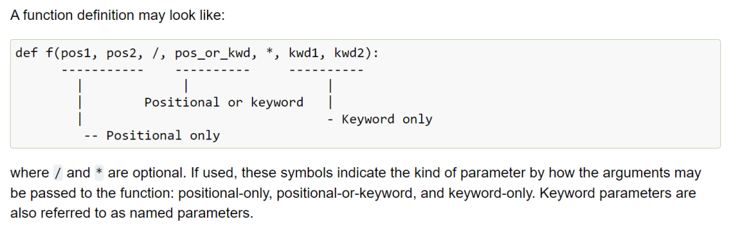
Hope C++’ll eventually come up with a compile-time contract syntax (method access control) that allows users to define what methods are allowed to touch which data member (potentially read/write as well) such as:

private:
   bool a : method1, method2(r), method3(w)
   char b : method2(rw), method3(r)

I don’t think we need to go that far to micromanage the other direction where methods declare which data members it could touch, as it needs extra work to check if the two directions agree. It’s methods that could go rogue on data. Data could not go rogue on methods unless they were abused/poisoned.

---

When to use classes

OOP is a useful idea but I would not over-objectify, like writing a class that holds 5 constants or organize a collection of loosely coupled or unrelated generic helper functions into a class (it should be organized into packages or namespaces). Over-objectifying reeks cargo cult programming.

My primary approach to program design is self-documenting. I prefer present the code in a way (not just syntax, but the architecture and data structure) that’s the easiest to understand without material sacrifices to performance or maintainability. I use classes when the problem statement happened to naturally align with the features classes has to offer without a lot of mental gymnastics to frame it as classes.

My decision process goes roughly like this:

• If a problem naturally screams data type (like matrices), which is heady on operator overloading, I’d use classes in a heartbeat as data types are mathematical objects.
• Then I’ll look into whether the problem is heavy on states. In other words, if it’s necessary for one method to drop something in the mailbox for another method to pick it up without meeting each other (through parameter passing calls), I’ll consider classes.
• If the problem statement screams natural interactions between objects, like a chess on the chessboard, I’d consider classes even if I don’t need OOP-specific features

---

Do not abuse OOP to hide bad practices

The last thing I want to use OOP as a tool for:

1. Hiding sloppy generic methods that is correct only given the implicit assumptions (specific to the class) that are not spelt out, like sorting unique 7 digit phone numbers.
2. Abusing data members to sugarcoat casually using globals and static all over the place (poor encapsulation) as if you’d have done it in a C program.

1) Free functions for generic operations

The first one is an example that calls for free functions. Instead of writing a special sort function that makes the assumption that the numbers are unique and 7 math digits. A free function bitmap_sort() should be written and put in a sorting library if there isn’t any off-the-shelf package out there.

In the process of refactoring parts of your program out into generic free functions (I just made up the word ‘librarize’ to mean this), you go through the immensely useful mental process of

• Explicitly understanding the exact assumptions that specifically applies to your problem that you want to take advantage of or work around the restrictions. You can’t be sure that your code is correct no matter how many tests you’ve written if you aren’t even clear about under what inputs your code is correct and what unexpected inputs will break the assumptions.
• Discover the nomenclature for the concept you are using
• Knowing the nomenclature, you have a very good chance of finding work already done on it so you don’t have to reinvent the wheel … poorly
• If the concept hasn’t been implemented yet, you can contribute to code reuse that others and your future self can take advantage of.
• Decoupling generic operation from business logic (the class itself) allows you to focus on your problem statement and easily swap out the generic implementation, whether it’s for debugging or performance improvement, or hand the work over to others without spending more time explaining what you wanted than writing the code yourself.

This is much better than jumping into writing a half-assed implementation of an idea that you haven’t fully understood the quirks (assumptions) and hide it as an internal method.

Decouple, decouple, decouple

By hiding the good stuff (a generic piece of code which is a useful algorithm) inside the class, you are merely luring the people dealing with your code base to go all the way out to break your intended access controls in order to get to the juicy implementation.

Don’t be embarassed if your first attempt in the generic code/algorithm is primative and it applies to very narrow input conditions! Instead of hiding the ’embarssing’ implementation inside a class that tolerates it due to the assumptions given the class’s context, you can simply add suffix to your function names to explain the limitations.

Making the name longer discourages people from expand its usage beyond what you intended. It also helps code reviewers catch people using your function when the restrictions denoted by the suffix of the function name clearly doesn’t apply to the said use.

Later on when people develop a more generic version (likely by learning from you), they can make the function name shorter after removing the restriction suffix. If your function turned out to be more generic than you’ve planned for, they can always write a wrapper that calls your function under the hood.

For example, during your exploration, you could start with sort_unique_phone_numbers() in your library. Later on somebody expanded on it and call it sort_unique_numbers(). Eventually some of you realized it’s bitmap_sort(). This way you don’t have to worry about colliding with the name sort() which is way more general.

If you factor the juicy implementation (of a generic idea) out of your class, others can happily use your library of free functions, leaving your internal implementations alone instead of trying questionable maneuvers to exploit it which lead to code cruft and debugging hell.

You learn a new concept well rather than repeating similar gruntwork over and over and it doesn’t benefit anybody else, and you likely have to debug the tangled mess when you run into a corner case because you didn’t understand the assumptions well enough to decouple a generic operation from the class.

Overload free functions!

Polymorphism in OOP is a lot broader than just function overloading.

virtuals has to be an OOP thing because it’s is run-time polymorphism, which make sense only with inheritance.

Templates (which also applies to free functions), and function overloading (which also applies to free function) are compile-time polymorphism.

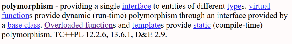
Polymorhpishm isn’t exclusive to OOP the way Bajrne defined it. C++ can overload free functions! You don’t need to put things into classes just because you want a context (signature) dependent dispatch (aka compiler figuring which version of the function with the same name to call).

I frequently overload free functions in MATLAB (by the type of the first argument) so it sound natural to me.

---

Program organization strategies

If you are really edgy about namespace pollution, just use namespace (but not class) for your free functions.

Here’s an example where I put half-baked generic library functions in C_tools and free functions that exclusively deal with the said class as C_free:

#include <iostream>

namespace C_tools { 
  int double_singleton(int x) { return 2*x; }
};

class C {
  public:
    C() : a(64) {}
    void update(int x) { a = x; }
    int a_doubled() { return C_tools::double_singleton(a); }
    int get_a() { return a; }
  private:
    int a;
};

namespace C_free {
  // It's a reference, so this changes the state
  void double_a(C& c) {
    c.update(c.a_doubled());
  }
};

int main() {
    C c; // Internally a is 64
    // a_doubled() returns the 2*a, giving 128
    std::cout << c.a_doubled() << std::endl;

    // Free generic helpers for others to use too
    // 2*89 = 178
    std::cout << C_tools::double_singleton(89) << std::endl;

    // Free functions acting on instances
    C_free::double_a(c);  // a=2*64=128
    std::cout << c.get_a() << std::endl;
    C_free::double_a(c);  // a=2*128=256
    std::cout << c.get_a() << std::endl;
    return 0;
}

The same namespace can be scattered in your code. So you can order them by the dependency in your code. There’s no reason to forward declare to keep the same namespace in one block.

I intentionally didn’t overload a free function in the example above to show that if your code is not really up to par to be generalized alongside with other code with the same idea and same name, it’s better to just use different names and not let C++ dispatch by context/signature.

In the following example,

• I merged C_tools to C_free to demonstrate that the same namespaces do not have to stay in one block. (Despite separating the two namespaces intended for different set of audience is a better practice)
• Now I merged C_tools are merged into C_free, I’ll take advantage of it to demonstrate free function overloading. Now there are two candidates of C_free:sqaure(): one takes an int while the other takes in a reference to class C, aka class C&.

#include <iostream>

namespace C_free { 
  int square(int x) { return x*x; }
};

class C {
  public:
    C() : a(64) {}
    void update(int x) { a = x; }
    int a_squared() { return C_free::square(a); }
    int get_a() { return a; }
  private:
    int a;
};

namespace C_free {
  // It's a reference, so this changes the state
  void square(C& c) {
    c.update(c.a_squared());
  }
};

int main() {
    C c; // Internally a is 64
    std::cout << c.a_squared() << std::endl; // 64*64=4096

    // Free generic helpers for others to use too
    std::cout << C_free::square(89) << std::endl; // 89*89=7921

    // Free functions acting on instances
    C_free::square(c);  // c.a=64*64=4096
    std::cout << c.get_a() << std::endl;
    C_free::square(c);  // c.a=4096*4096=16777216
    std::cout << c.get_a() << std::endl;
    return 0;
}

2) Classes are not excuses to hide unnecessary uses of global/statics

Data members in classes are namespace-scoped version of global/static variables that could be optionally localized/bound to instances. Private/Public access specifiers in C++ expanded on global/file scope variables switched through static modifier (file scope) back in C days.

If you don’t think it’s a good habit to sprinkle global scope all over the place in C, try not to go wild using more data members than necessary either.

Data members give an illusion that you are encapsulating better and ended up incentivising less defensive programming practices. Instead of not polluting in the first place (designing your data flow using the mentality of global variables), it merely contained the pollution with namespace/class scopes.

For example, if you want to pass a message (say an error code) directly from one method to another and NOBODY else (other methods) are involved, you simply pass the message as an input argument.

Globals or data members are more like a mechanism that you drop a letter to a mailbox instead of handing it your intended recipient and hope somehow the right person(s) will reach it and the right recipient will get it. Tons of things can go wrong with this uncontrolled approach: somebody else could intercept it or the intended recipient never knew the message is waiting for him.

With data members, even if you marked them as private, you are polluting the namespace of your class’s scope (therefore not encapsulating properly) if there’s any method that can easily access data members that it doesn’t need.

---

How I figured this out on my own based on my experience in MATLAB

Speaking of insidious ways to litter your program design the globalist mentality (pun intended), data members are not the only offenders. Nested functions (not available in C++ but available in modern MATLAB and Python) is another hack that makes you FEEL less guilty structuring your program in terms of global variables. Everything visible one level above the nested function is relatively global to the nested function. You are literally polluting the variable space of the nested function with local variables of the function one level above, which is a lot more disorganized than data members that you kind of acknowledge what you’ve signed up for.

Librarize is the approach I came up with for MATLAB development: keep a folder tree of user MATLAB classes and free functions organized in sensible names. Every time I am tempted to reinvent the wheel, I try to think of the best name for it. If the folder with the same name exist, chances are I already did something similar before and just needed a little reminder. This way I always have high quality in-house generic functions (which I could expand the use cases with backward compatibility as needed).

This approach works because I’m confident with my ability to naturally come up with sensible names consistently. When I did research in undergrad, the new terminologies I came up with happened to coincide with wavelets before I studied wavelets, as in hindsight what I was doing was pretty much the same idea as wavelets except it doesn’t have the luxury of orthogonal basis.

If a concept has multiple names, I often drop breadcrumbs with dummy text files suggesting the synonym or write a wrapper function with a synonymous name to call the implemented function.

C++ could simply overload free functions by signatures, but not too many people know MATLAB can overload free functions too! MATLAB’s function overload is polymorphic (the decision on which version to dispatch) by ONLY BY THE FIRST ARGUMENT.

MATLAB supports variable arguments which defeats the concept of signatures. So be grateful that at least it can overload by the first argument. Python doesn’t even overload by the first arugment.

It’s a very advanced technique I came up with which allow the same code to work for many different data types, doing generics without templates available in C++.

I also understand that commercial development are often rushed so not everybody could afford the mental energy to do things properly (like considering free functions first). All I’m saying is that there’s a better way than casually relying on data members more than needed, and using data member should have the same stench as using global variables: it might be the right thing to do in some cases, but most often not.

If you see people sticking to free functions, please consider the merits of it before jumping to judging them. It’s easy to tell based on the application (based on how ‘hard’ they try, aka bending things to fit a paradigm) if people are doing things one way or the other religiously or they adapt to the problem they are solving.